Time Series Forecasting 3 - Multi-step Forecasting
This is Part 3 in a series on time series forecasting - The full series is Part 1, Part 2, and Part 3.
This post covers how to do multi-step or open-loop forecasting using the data mining approach presented in Part 1 of this series. As described in Part 1, multi-step forecasting allows making predictions for more time steps in the future than single-step forecasting. Unlike single-step forecasting (Part 2), the recursive nature of multi-step forecasting cannot be computed via the SQL PREDICTION function alone. However, we can compute multi-step forecasts using the SQL PREDICTION function within a SQL MODEL clause. Below I describe how this is done and illustrate the approach with two examples.
Methodology
Multi-step forecasting requires the same methodology for developing a model as the one described in Part 1 and detailed in Part 2. The only difference is how we score the model.
Forecasting
Consider a sales time series (ts_data) with daily sales figures for the first seven days (Figure 1).
Figure 1: Sales data.
Consider also that, following the methodology outlined in Part 1 and Part 2, we have created a data mining regression model (ts_model) that can be used for forecasting future sales based on the sales of the previous seven days. We would like to predict the sales for the next seven days (days 8 through 14) using the ts_model. As shown in Part 2, it is possible to use the PREDICTION SQL function for single step ahead forecast. For the present example, the following query produces one-step ahead forecasts:SELECT day, sales,
PREDICTION(ts_model USING
LAG(sales,1) OVER (ORDER BY day) as l1,
LAG(sales,2) OVER (ORDER BY day) as l2,
LAG(sales,3) OVER (ORDER BY day) as l3,
LAG(sales,4) OVER (ORDER BY day) as l4,
LAG(sales,5) OVER (ORDER BY day) as l5,
LAG(sales,6) OVER (ORDER BY day) as l6,
LAG(sales,7) OVER (ORDER BY day) as l7
) pred
FROM ts_data a;
Because the model requires the sales of the previous seven days as inputs, initially we can only obtain a forecast for day 8 sales. For forecasting sales for days 9 through 14, we would need to run this query at the end of every day, once the day's sales are available, to forecast the sales for the next day. Although this provides some useful information it does not allow much time for planning. Ideally we would like to generate forecasts for the next seven days at once. Here comes multi-step forecasting to the rescue. In multi-step forecasting we use actual series values when available and previously forecasted values when the actual values are not available. We also create new rows. That is, we create predictions for rows with day values not present in the input data set. The result data set should look like the one in Figure 2.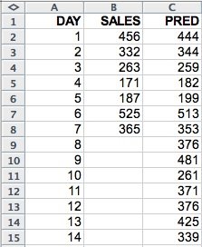
Figure 2: Multi-step forecast for the sales data.
Multi-Step Multi-step Forecasting - No Transformation CaseWe can generate multi-step forecasts using the SQL PREDICTION function within a SQL MODEL clause. For this example we can use the following query:
SELECT d day, s sales, p predThe SQL MODEL clause defines a multidimensional spreadsheet-like view of the data. The dimensions index the rows of the spreadsheet and measures are the columns. The RULES statement allows the definition of computation rules for each column for the specified row ranges. If the specified range goes beyond the actual range in the data new rows are inserted. For good introductions to the SQL MODEL clause see "The SQL Model Query of Oracle 10g" white paper and the "Announcing the New Model" article.
FROM ts_data a
MODEL
DIMENSION BY (day d)
MEASURES (sales s, CAST(NULL AS NUMBER) p)
RULES(
p[FOR d FROM 1 TO 14 INCREMENT 1] =
PREDICTION(ts_model USING
NVL(s[CV()-1], p[CV()-1]) as l1,
NVL(s[CV()-2], p[CV()-2]) as l2,
NVL(s[CV()-3], p[CV()-3]) as l3,
NVL(s[CV()-4], p[CV()-4]) as l4,
NVL(s[CV()-5], p[CV()-5]) as l5,
NVL(s[CV()-6], p[CV()-6]) as l6,
NVL(s[CV()-7], p[CV()-7]) as l7)
)
ORDER BY d
For multi-step forecasting using the SQL MODEL clause, we need to define a prediction measure. This measure is computed using the PREDICTION SQL function and a range that includes the historical period as well as the forecast period. The computation should use actual values as inputs when available and previously predicted values when no actual inputs are available. The latter is the case for the forecast period.
Let's analyze the query piece by piece. The query specifies a "spreadsheet" view of the data like that represented in Figure 2. The DIMENSION clause indicates that the rows are indexed by the column day. The MEASURES clause defines two measures: the original sales and a column pred, initialized to NULL, to hold the predictions. The RULES clause indicates how to compute the column pred, the predictions, for d (day dimension) going from 1 to 14 in increments of 1. The range 8-14 is not present in the original data and is the forecast period. The rule for pred uses the PREDICTION function to compute the predictions. The NVL function returns the value for sales for a given d value if that value is not NULL, otherwise it returns the value in the prediction column pred. The syntax s[CV()-1] specifies the sales (s) value for the previous day. For example, for d=7 then s[CV()-1] represents the sales for d=6. This notation provides a convenient way to specify the lagged values required as inputs to time series forecasting models.
Often, we want to compute multi-step forecasts for periods where we do have the actual values for the time series. This is the case when we are trying to assess model quality. In such cases, we can modify the above query in the following way:
SELECT d day, s sales, p pred
FROM ts_data a
MODEL
  DIMENSION BY (day d)
  MEASURES (sales s, CAST(NULL AS NUMBER) ap,
            CAST(NULL AS NUMBER) p)
  RULES(
    ap [FOR d FROM 1 TO 7 INCREMENT 1] = s[CV()],
    p[FOR d FROM 1 TO 14 INCREMENT 1] =
              PREDICTION(ts_model USING
                         NVL(ap[CV()-1], p[CV()-1]) as l1,
                         NVL(ap[CV()-2], p[CV()-2]) as l2,
                         NVL(ap[CV()-3], p[CV()-3]) as l3,
                         NVL(ap[CV()-4], p[CV()-4]) as l4,
                         NVL(ap[CV()-5], p[CV()-5]) as l5,
                         NVL(ap[CV()-6], p[CV()-6]) as l6,
                         NVL(ap[CV()-7], p[CV()-7]) as l7)
  )
ORDER BY d
This query specifies a "spreadsheet" view of the data like the one in Figure 3. The MEASURES clause defines three measures: the original sales, an auxiliary column ap, and a column p to hold the predictions initialized to NULL. ap is introduced to represent the "historical" period for the time series. It takes on the values of the original series for the training period and is left undefined (NULL) for the forecast period. This simple modification to the original query allows keeping the structure of the rest of the query the same. Note that we also replaced s with ap in the rules.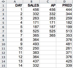
Figure 3: Multi-step forecast for the sales data, validation case.
Once the predictions have been computed we can assess the quality of a model by comparing the predicted and actual values for the series over the forecasting range. Typical measures include: Root Mean Square Error (RMSE), Mean Absolute Error (MAE), Mean Absolute Percentage Error (MAPE), and maximum error. For example, the RMSE error for the data in Figure 3 computed for day between 8 and 14 is 11.18.Multi-Step Multi-step Forecasting - Transformation Case
If the data has to be transformed before model building (see Part 2 for an example) then the transformations need to be included in the query computing the forecasts. Consider that, like the airline example in Part 2 we had to LOG transform, differencing, and normalize (z-score) the sales data in order to build the ts_model regression model. We would need to modify the above query as follow:
SELECT d day, s sales, p predThe query defines a "spreadsheet" view of the data like that represented in Figure 4. The DIMENSION clause indicates that the rows are indexed by the column day. The MEASURES clause defines the following measures:
FROM ts_data a
MODEL
DIMENSION BY (day d)
MEASURES (sales s, CAST(NULL AS NUMBER) ts,
CAST(NULL AS NUMBER) tp, CAST(NULL AS NUMBER) np,
CAST(NULL AS NUMBER) dp, CAST(NULL AS NUMBER) p)
RULES(
ts[FOR d FROM 1 TO 14 INCREMENT 1] =
(LOG(10,s[CV()]) - LOG(10,s[CV()-1]) + 0.010578734)/0.193587249,
tp[FOR d FROM 1 TO 14 INCREMENT 1] =
PREDICTION(ts_model USING
NVL(ts[CV()-1], tp[CV()-1]) as l1,
NVL(ts[CV()-2], tp[CV()-2]) as l2,
NVL(ts[CV()-3], tp[CV()-3]) as l3,
NVL(ts[CV()-4], tp[CV()-4]) as l4,
NVL(ts[CV()-5], tp[CV()-5]) as l5,
NVL(ts[CV()-6], tp[CV()-6]) as l6,
NVL(ts[CV()-7], tp[CV()-7]) as l7),
np[FOR d FROM 1 TO 14 INCREMENT 1] =
0.193587249 * tp[CV()] - 0.010578734,
dp[FOR d FROM 1 TO 14 INCREMENT 1] =
np[CV()] + NVL(LOG(10,s[CV()-1]),dp[CV()-1]),
p[FOR d FROM 1 TO 14 INCREMENT 1] = POWER(10,dp[CV()])
)
ORDER BY d
- sales is the original sales data
- ts represents the data after all the transformations, in order: LOG transform, differencing, and z-score normalization.
- tp contains the predicted values for the training and the forecasting period. The predictions are provided in the same scale as the transformed data
- np reverses the normalization transformation on the predicted values
- dp reverses the differencing transformation step
- p is the prediction on the same scale of the original, untransformed, sales series, after reversing the effects of the LOG transformation using the POWER function
For clarity, I broke down each reverse transformation step into its own measure. This is not necessary, but it makes it easier to illustrate how each transformation can be reversed. Basically for each transformation performed in the original series we can introduce a reverse transformation step that will "reverse transform" the predicted values until they are in the same scale of the original data. The above query illustrates most of the transformation we would need to use in time series modeling following the methodology presented in Part 1 and Part 2. The query also showcases the power of the SQL MODEL clause. The MODEL clause enables the definition of multiple computations in a clear and concise form.
Figure 4: Multi-step forecast for the sales data, transformation case.
If we did have the actual values for the time series for the forecast period we would again introduce a new measure ap and replace s with ap in all the rules. The modified query would look like this:SELECT d day, s sales, p predExample 1: Airline Passengers Forecast
FROM ts_data a
MODEL
DIMENSION BY (day d)
MEASURES (sales s,
CAST(NULL AS NUMBER) ap, CAST(NULL AS NUMBER) ts,
CAST(NULL AS NUMBER) tp, CAST(NULL AS NUMBER) np,
CAST(NULL AS NUMBER) dp, CAST(NULL AS NUMBER) p)
RULES(
ap [FOR d FROM 1 TO 7 INCREMENT 1] = s[CV()],
ts[FOR d FROM 1 TO 14 INCREMENT 1] =
(LOG(10,ap[CV()]) - LOG(10,ap[CV()-1]) + 0.010578734)/0.193587249,
tp[FOR d FROM 1 TO 14 INCREMENT 1] =
PREDICTION(ts_model USING
NVL(ts[CV()-1], tp[CV()-1]) as l1,
NVL(ts[CV()-2], tp[CV()-2]) as l2,
NVL(ts[CV()-3], tp[CV()-3]) as l3,
NVL(ts[CV()-4], tp[CV()-4]) as l4,
NVL(ts[CV()-5], tp[CV()-5]) as l5,
NVL(ts[CV()-6], tp[CV()-6]) as l6,
NVL(ts[CV()-7], tp[CV()-7]) as l7),
np[FOR d FROM 1 TO 14 INCREMENT 1] =
0.193587249 * tp[CV()] - 0.010578734,
dp[FOR d FROM 1 TO 14 INCREMENT 1] =
np[CV()] + NVL(LOG(10,ap[CV()-1]),dp[CV()-1]),
p[FOR d FROM 1 TO 14 INCREMENT 1] = POWER(10,dp[CV()])
)
ORDER BY d
Let's use the airline_SVM model described in Part 2 for multi-step forecasting and compare the results with those for one-step ahead forecasting. The following query generates predictions for both the training data and the 12 months forecasting (month index 132 to 144):
SELECT m month, p passengers, predAs we have the actual values for the series for the forecasting period and we transformed the data before building the model, I used the validation with transformation version of the scoring query described above. Again I broke down each transformation step into its own measure. The RULES section details how to compute each of the measures:
FROM airline a
MODEL
DIMENSION BY (month m)
MEASURES (a.passengers p,
CAST(NULL AS NUMBER) ap, CAST(NULL AS NUMBER) tp,
CAST(NULL AS NUMBER) tpred, CAST(NULL AS NUMBER) npred,
CAST(NULL AS NUMBER) dpred, CAST(NULL AS NUMBER) pred)
RULES(
ap [FOR m FROM 1 TO 131 INCREMENT 1] = p[CV()],
tp[FOR m FROM 1 TO 131 INCREMENT 1] =
(LOG(10,ap[CV()]) - LOG(10,ap[CV()-1]) - 0.003919158)/0.046271162,
tpred[FOR m FROM 1 TO 144 INCREMENT 1] =
PREDICTION(airline_SVM USING
NVL(tp[CV()-1],tpred[CV()-1]) as l1,
NVL(tp[CV()-2],tpred[CV()-2]) as l2,
NVL(tp[CV()-3],tpred[CV()-3]) as l3,
NVL(tp[CV()-4],tpred[CV()-4]) as l4,
NVL(tp[CV()-5],tpred[CV()-5]) as l5,
NVL(tp[CV()-6],tpred[CV()-6]) as l6,
NVL(tp[CV()-7],tpred[CV()-7]) as l7,
NVL(tp[CV()-8],tpred[CV()-8]) as l8,
NVL(tp[CV()-9],tpred[CV()-9]) as l9,
NVL(tp[CV()-10],tpred[CV()-10]) as l10,
NVL(tp[CV()-11],tpred[CV()-11]) as l11,
NVL(tp[CV()-12],tpred[CV()-12]) as l12),
npred[FOR m FROM 1 TO 144 INCREMENT 1] =
0.003919158 + 0.046271162 * tpred[CV()],
dpred[FOR m FROM 1 TO 144 INCREMENT 1] =
npred[CV()] + NVL(LOG(10,p[CV()-1]),dpred[CV()-1]),
pred[FOR m FROM 1 TO 144 INCREMENT 1] = POWER(10,dpred[CV()])
)
ORDER BY m;
- ap takes on the values of the original series for the training period (1 to 131) and is left undefined (NULL) for the forecast period (132 to 144)
- tp transforms the data, in order: LOG transform, differencing, and z-score normalization.
- tpred computes the predicted values for the training and the forecasting period using the PREDICTION function. The rule uses the actual transformed values for the series (tp) when available; otherwise it uses the previous predictions. The predictions are provided in the same scale as the transformed data
- npred reverses the normalization transformation on the predicted values
- dpred reverses the differencing transformation step. It uses the actual value for the series if available, otherwise it uses the previous value for dpred. Because, when building the model, differencing followed a LOG transformation, when using the actual values we need to LOG transform the series.
- pred is the prediction on the same scale of the original (untransformed) series after reversing the effects of the LOG transformation by applying the POWER function.
Figure 5 shows the original data, the model multi-step predictions, and the residuals for the whole series (month 1-144). Due to the use of first order differencing, we do not have a prediction for the first time period (month 1).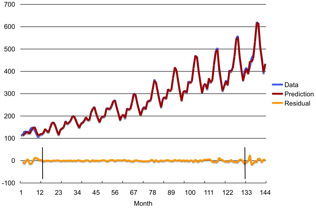
Figure 5: Data, multi-step predictions, and residuals.
The two vertical bars in the residual series mark the beginning and the end of the samples used for training the model. Samples to the left of the first bar contain NULL values for some of the lagged variables used as inputs to the model. The predictions for this period are a bit off as some of the inputs are missing. The interval to the right of the second bar is the forecasting period. Samples in this interval are the held aside samples used for measuring the model's generalization capabilities. Note that the model output for these samples are multi-step ahead forecasts of data unseen during training of the model.
As illustrated by the picture, the model ability to generate multi-step forecasts is very good. How well does the data mining approach described above compare with other techniques and the one-step ahead forecast approach? Table 1 presents the Root Mean Squared Error (RMSE) and Mean Absolute Error (MAE) for the training and the forecast (test) data sets for the data mining approach (SVM) and a linear autoregressive model (AR) using one-step and multi-step forecasting approaches.
| Model | RMSE Training | MAE Training | RMSE Test | MAE Test |
| SVM (one-step) | 3.7 | 3.2 | 18.9 | 13.4 |
| AR (one-step) | 10.1 | 7.7 | 19.3 | 15.2 |
| SVM (multi-step) | 3.7 | 3.2 | 11.5 | 9.3 |
The SVM multi-step approach performed well. It had a smaller RMSE and MAE in the forecasting (test) data set than the AR and the SVM models used in one-step forecasting mode.
Example 2: Electric Load Forecast
In this example, the problem to be solved is the forecasting of maximum daily electric load based on previous electric load values and additional data. The training data consist of half an hour loads for the time period 1997 – 1998. The goal is to supply the prediction of maximum daily values of electric loads for January 1999 (31 data values altogether). This data was used in a electric load forecasting competition. The data, the competition submissions, and results are here.
The winning entry by Lin used the support vector machine regression algorithm. In this example, I closely followed Lin's approach as described here. Like Lin, I used the following inputs to build the model:
- The seven previous maximum load values
- The day of the week
- A 0-1 flag indicating if it is a holiday or not
First, I combined the data from the different files (1997, 1998, 1/1999) into a single file and then loaded the data into the table load_all with schema (day_id NUMBER, day DATE, day_week VARCHAR2(1), max_load NUMBER, holiday NUMBER), where the day_id column is a sequence ranging from 1 to 761 going up with day, and day_week is the day of the week for a given day. day_week can be easily computed as TO_CHAR(day,'d'). Figure 6 shows the maximum load values for load_all.
Figure 6: Maximum daily electric load from 1/1/97 to 1/31/99.
Because the series does not have any obvious trends on its mean or variance (see Part 2), we only need to normalize the max_load column in order to prepare the data for building a model. Like Lin, I normalized the series to the [0,1] range as follow:
CREATE VIEW load_norm AS
SELECT day_id, day, max_load, holiday, day_week,
       (max_load-464)/(876-464) tl
FROM load_all
where 464 and 876 are, respectively, the MIN(max_load) and MAX(max_load) for the 1/1/97 to 12/31/98 period.
Before building a model we need to select which lag values of the prepared series to use as predictors of future values. As discussed in Part 2, this is equivalent to selecting a time window and including all the lag values in that window. Prior knowledge about the activity represented by the series can provide an initial clue. It is also useful to analyze the autocorrelations in the series and chose a window size that includes the largest autocorrelation terms.
Autocorrelations can be easily computed using the xcorr procedure introduced in Part 2. The autocorrelation of the tl series with its first 20 lags can be computed as follow:
BEGIN
  xcorr(p_in_table  => 'load_norm',
        p_out_table => 'my_corr',
        p_seq_col   => 'day_id',
        p_base_col  => 'tl',
        p_lag_col   => 'tl',
        p_max_lag   => 20);
END;
/
Figure 7 shows the first twenty autocorrelations coefficients for the electric load series. The largest autocorrelation term is at lag 7. This seems reasonable, as we would expect electric load to display a strong weekly seasonal effect. Based on this analysis, we may want to include as predictors all the lags in a window of size 7.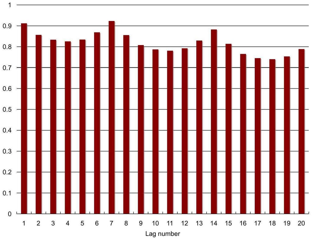
Figure 7: First twenty autocorrelation coefficients for the electric load series.
After normalizing the series and selecting the lagged variables we are ready to build a model to forecast future values of the series. First we need to create a view with the seven lagged variables:CREATE VIEW load_lag asNext we create the training dataset as a subset of the rows in load_lag. Because we want to test the model's forecasting capability we should train on older data samples and held aside, for testing, the most recent samples in the series. Samples 731-761 are used for the test data set. We also need to filter the first 7 rows as some of the lagged variables have NULLs for these rows. Unlike Lin, I decided to include the months of August and September in the training data as well. The following view creates the training data set:
SELECT day_id, day, max_load, tl, holiday, day_week,
LAG(tl, 1) OVER (ORDER BY day) L1,
LAG(tl, 2) OVER (ORDER BY day) L2,
LAG(tl, 3) OVER (ORDER BY day) L3,
LAG(tl, 4) OVER (ORDER BY day) L4,
LAG(tl, 5) OVER (ORDER BY day) L5,
LAG(tl, 6) OVER (ORDER BY day) L6,
LAG(tl, 7) OVER (ORDER BY day) L7
FROM load_norm
CREATE VIEW load_train ASFinally we build the model using either Oracle Data Miner or one of the data mining APIs. For this example, I used the PL/SQL API and the default settings for the SVM regression algorithm:
SELECT day_id, day, max_load, tl, holiday, day_week,
L1, L2, L3, L4, L5, L6, L7
FROM load_lag
WHERE day_id < 731 and day_id > 7;
BEGIN
  DBMS_DATA_MINING.CREATE_MODEL(
    model_name          => 'load_SVM',
    mining_function     => dbms_data_mining.regression,
    data_table_name     => 'load_train',
    case_id_column_name => 'day_id',
    target_column_name  => 'tl');
END;
This statement creates an SVM regression model named load_SVM using the view load_train as the training data.
Figure 8 displays the residual plot for the training data. The residuals are computed as the difference between the prediction and the actual value for the series. Ideally we want the residuals (Y-axis values) to be randomly distributed around zero with no discernible trends. The plot shows that the model does a good job capturing the process underlying the time series.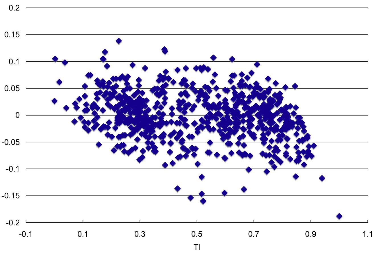
Figure 8: Residual plot.
To create forecasts we only need to apply the model to new data. For example, applying the load_SVM model to the load_lag view generates multi-step ahead forecasts for both the training data (samples 1-730) as well as the held aside test data (samples 731-761). The following query accomplishes that:
SELECT m day_id, p max_load, pred
FROM load_all a
MODEL
  DIMENSION BY (day_id m)
  MEASURES (a.max_load p, a.day_week dw, a.holiday h,
            CAST(NULL AS NUMBER) ap, CAST(NULL AS NUMBER) tp,
            CAST(NULL AS NUMBER) tpred,
            CAST(NULL AS NUMBER) pred)
  RULES(
    ap [FOR m FROM 1 TO 730 INCREMENT 1] = p[CV()],
    h[FOR m FROM 731 TO 761 INCREMENT 1] = 0,
    tp[FOR m FROM 1 TO 730 INCREMENT 1] =
              (ap[CV()] - 464)/(876-464),
    tpred[FOR m FROM 1 TO 761 INCREMENT 1] =
              PREDICTION(load_SVM USING
                           NVL(tp[CV()-1],tpred[CV()-1]) as l1,
                           NVL(tp[CV()-2],tpred[CV()-2]) as l2,
                           NVL(tp[CV()-3],tpred[CV()-3]) as l3,
                           NVL(tp[CV()-4],tpred[CV()-4]) as l4,
                           NVL(tp[CV()-5],tpred[CV()-5]) as l5,
                           NVL(tp[CV()-6],tpred[CV()-6]) as l6,
                           NVL(tp[CV()-7],tpred[CV()-7]) as l7,
                           dw[CV()] as day_week,
                           h[CV()] as holiday
                ),
    pred[FOR m FROM 1 TO 761 INCREMENT 1] =
              464 + (876-464) * tpred[CV()]
  )
ORDER BY m;
This query follows the same structure of the other multi-step forecasting queries described above. Because normalization was the only transformation used to prepare the data, we only need a single to step for reversing transformations in the RULES section after the computation of the predictions. The main difference between this query and the previous ones is the addition of some extra measures to capture the inputs to the model that are not lagged variables, namely: day_week and holiday. Also, following Lin, I set the holiday flag (h) to zero for the forecasting period. This is done in the second rule in the query.
Figure 9 shows the original data, the model multi-step predictions, and the residuals from 1/1/97 to 1/31/99. The large error for the first day reflects the absence of previous values for the series in the inputs.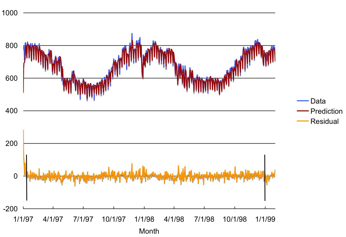
Figure 9: Data, multi-step predictions, and residuals.
The two vertical bars in the residual series mark the beginning and the end of the samples used for training the model. Samples to the left of the first bar contain NULL values for some of the lagged variables used as inputs to the model. The predictions for this period are a bit off as some of the inputs are missing. The interval to the right of the second bar is the forecasting period. Samples in this interval are the held aside samples used for measuring the model's generalization capabilities. Note that the model output for these samples are multi-step ahead forecasts of data unseen during training of the model.
Again, we would like to know how well does the data mining approach, described above, compare with other techniques and the one-step ahead forecast approach? Table 2 presents the Mean Absolute Percentage Error (MAPE) and the Maximum Load Error (MAX) for the training and the forecast (test) periods for the data mining approach (SVM) using one-step and multi-step forecasting approaches.
| Model | MAPE Training | MAX Load Error Training | MAPE Test | MAX Load Error Test |
| SVM (one-step) | 2.2 | 77.4 | 1.7 | 39.1 |
| SVM (multi-step) | 2.2 | 77.0 | 1.9 | 50.4 |
The SVM multi-step approach performed well. It had about the same MAPE but a somewhat larger MAX load forecast error than the one-step approach in the test period. Figures 10 and 11 show the actual and forecasted values for the test period (1/99) using the one-step and the multi-step approaches respectively.
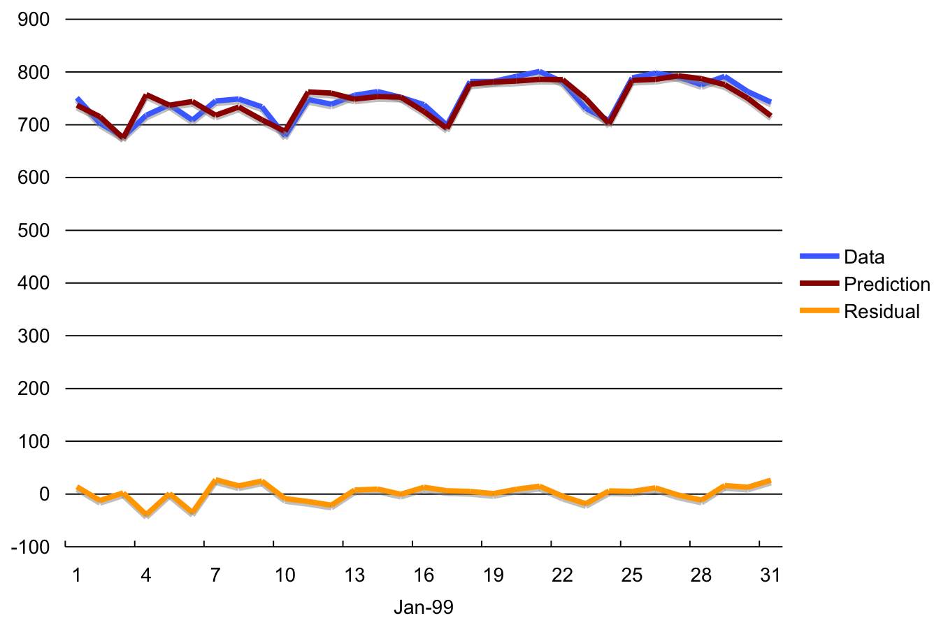
Figure 10: Data and one-step predictions for 1/99.

Figure 11: Data and multi-step predictions for 1/99.
Finally, Figure 12 shows how the results for our SVM multi-step approach compares with other methods, including: Adaptive Logic Network, Fuzzy Inference Systems, Neural Networks, Functional Networks, MARS, and Self-Organizing Maps. Because our results are similar to those obtained by Lin (dark circle), we case use those as a proxy for our results. However, it is important to notice that our results were obtained without the expensive cross-validation methodology used by Lin. This was possible because Oracle Data Mining SVM algorithm automatically tunes the SVM parameters to generate good results.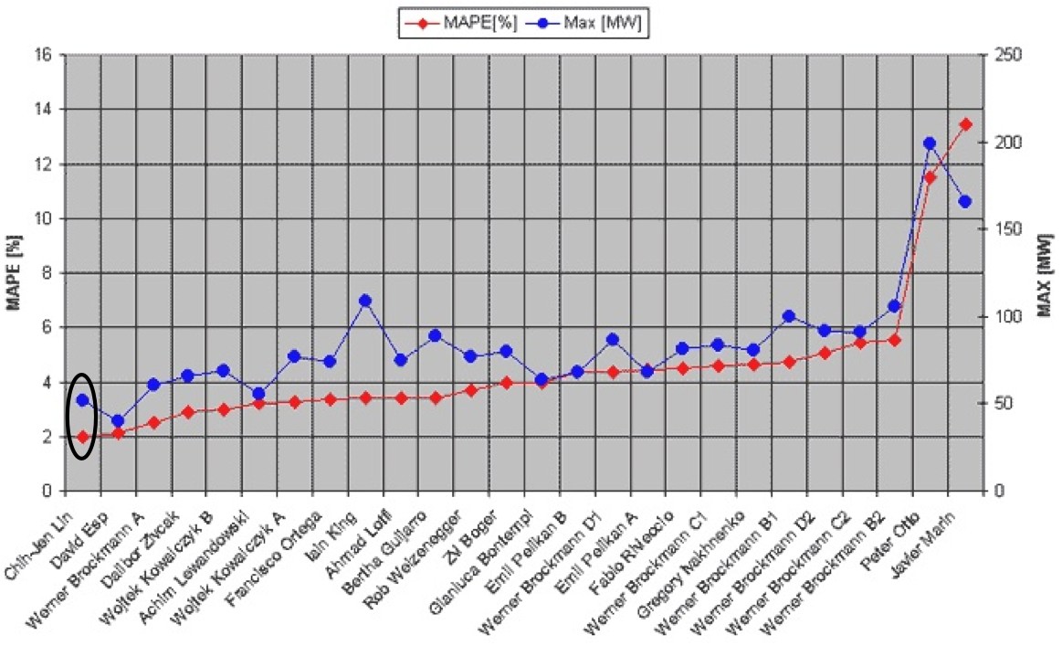
Figure 12: Electricity load forecast competition results (adapted from here).
Conclusions
This series outlined how we can use Oracle Data Mining to create powerful models for time series forecasting. The series described the methodological steps needed and illustrated the different approaches with well known time series examples. The Electric Load forecast problem also showed how other variables, besides past values of the time series, can be easily leveraged by the approach described in the series.
Drop me a note with your thoughts and/or experiences with the techniques described here.
10/26/06 - Edits
In the airline example described in Part 2, the normalization shift and scale parameters were computed using the whole data. A better methodology would be to use only the training data for computing these parameters. This alternative normalization scheme also impacts the results for the airline example described above as the latter builds on the transformations described in Part 2. I have changed the normalization in Part 2 so that the parameters are computed using only the training data time period. The above queries were also modified to reflect these new parameter values.
The results for the electric load forecast example did not reflect the respective forecasting query. They reflected an earlier version of the query. The correct results are a little better. The Max Load Error decreased from 77.4 to 77.0 for the training set and from 50.9 to 50.4 for the test set. I have replaced the old numbers with the new ones.
Links to a script for reproducing both examples and the respective data can be found here.
Labels: Time Series


I have posted a link to the script and the data in the Time Series Revisited post. Take a look at the Edits comments above. There is a link to that post there.
Posted by Marcos |
10/28/2006 07:16:00 PM
Marcos |
10/28/2006 07:16:00 PM
Amzing description
thanks a lot
Deepa
Posted by Anonymous |
2/07/2007 06:10:00 AM
Anonymous |
2/07/2007 06:10:00 AM
I've had great difficulty with my attempts at time-series modeling and prediction of a financial market index. Your entire three-part description of your methods has been quite helpful. You've directly and indirectly given me fresh ideas regarding choice of inputs, targets, and preparation of the training sets. Thanks very much!
Doug W.
Posted by Anonymous |
5/26/2007 12:41:00 AM
Anonymous |
5/26/2007 12:41:00 AM
Thanks Doug. Happy to hear that it helped.
Posted by Marcos |
5/27/2007 11:16:00 AM
Marcos |
5/27/2007 11:16:00 AM
This comment has been removed by a blog administrator.
Posted by Anonymous |
6/28/2007 09:28:00 PM
Anonymous |
6/28/2007 09:28:00 PM
Excellent description!
I am, however, confused as to how you can efficiently train the SVM based model frequently, when you get new data. Assuming you get new data every day...
For instance, we intially train in given a data set, i.e. segregate the set to training data and validation set... A process to teach and test and choose appropriate parameters to produce a very smart agent...
My quesiton is, do you not find the method to be inefficient in that you have to retrain the SVM evertime you recieve more data, and go through the entire process of stabilizing the variance, normalizing the targets, defining lagged variables, etc... Do we just do this on a predefined frequency or is there a way for us to train it given historical data, and just keep feeding it new data as it comes?
Similar to an online neural network that is trained with new examples as opposed to a batched learing approach...
Posted by Anonymous |
6/28/2007 09:29:00 PM
Anonymous |
6/28/2007 09:29:00 PM
It all depends on how frequently you want to train your model. Let say you receive new data every minute and you want to make predictions for a number of minutes ahead taking into account the new data. The described method would be inefficient in this case. An online neural network could handle this better but you would need to be careful regarding model stability and avoiding overfitting the new data. In other words, if you trained the network in batch you would get a different result from training it incrementally on the same data.
For the example you gave, receiving new data on a daily base, I don't see a problem. ODM SVM implementation with active learning train very quickly. In fact even if you had new data every hour it would not be a problem.
Something else to keep in mind is that, in many real systems, there is a lag between modifying models and placing them in production. Unless you have algorithms that are incrementally stable (e.g., Naive Bayes), I don't think that one should have a incremental (online) learning algorithm in production. It would be a risky proposition.
Posted by Marcos |
7/14/2007 02:01:00 AM
Marcos |
7/14/2007 02:01:00 AM