Bioinformatics the SQL Way
It is not uncommon for Bioinformatics data to have a large number of numeric attributes. For example, DNA microarray data can have thousands of attributes (gene expression values) per sample. The large number of attributes poses special challenges for the storage and analysis of microarray data. I have been asked, a number of times, what could be done to facilitate working with this type of data in the database. In this post I show, through a series of examples based on a well-known DNA microarray data set, how SQL can be used to address data load and representation, data transformation, and gene filtering.
The Data
For the examples below, I took a subset of the DNA microarray data used in the paper "Diffuse Large B-Cell Lymphoma Outcome Prediction by Gene Expression Profiling and Supervised Machine Learning" (Shipp et al, 2002). The data I used come in two files and can be download here: lymphoma_8_lbc_outcome_rn.res and lymphoma_clinical_011127.xls. The first file contains gene expression values in Affymetrix's scaled average difference units. These average difference values were generated by Affymetrix's GeneChip software. There are 7129 attributes and 58 samples. Because of the large number of attributes, the attributes are represented as rows and the samples as columns. The second file is a Microsoft Excel worksheet containing clinical information for the Lymphoma samples used in the study. This table cross references the sample identifier with the full International Prognosis Index (FULL_IPI), the patient's survival time in moths from diagnosis to the latest follow-up (SURTIME), the patient's current (at last follow-up) disease status (STATUS), and the outcome class (OUTCOME). An OUTCOME with value of 0 indicates a Diffuse Large B-Cell Lymphoma (DLBCL) sample from a cured patient while a 1 indicates a DLBCL sample from a patient with fatal or refractory disease. This type of data can be used for predictive analysis such as uncovering the most important factors (genes) in determining a positive or negative outcome for a treatment.
Data Load and Representation
Let's say that we want to represent the Lymphoma data in the database in three tables (schemas are in parenthesis):
- lymph_outcome (sample_id VARCHAR2(6), full_ipi VARCHAR2(20), surtime NUMBER, status VARCHAR2(20), outcome VARCHAR2(1)) stores clinical data, specially the outcome for each sample. A zero indicates a positive outcome (cured) and a 1 a negative outcome (fatal).
- lymph_exp (sample_id VARCHAR2(6), gene_id NUMBER, gene_exp NUMBER) stores gene expression values for each sample. This is the data that comes from processing the DNA microarray chip.
- lymph_map (gene_id NUMBER, description CLOB, accession VARCHAR2(4000)) stores the mapping of gene descriptions to gene IDs created while loading the data.
- Export the Excel spreadsheet data to a tab delimited text file (lymph_clinical.dat)
- Create the tables needed to represent the Lymphoma data in the database
- Load the data
- Pivot the temporary gene expression table
DROP TABLE lymph_outcome PURGE;The table lymph_temp is a temporary table for holding the original gene expression data. In order to create the lymph_exp table we have to pivot this temporary table.
CREATE TABLE lymph_outcome (sample_id VARCHAR2(6),
full_ipi VARCHAR2(20),
surtime NUMBER,
status VARCHAR2(20),
outcome VARCHAR2(1));
DROP TABLE lymph_map PURGE;
CREATE TABLE lymph_map (gene_id NUMBER,
description CLOB,
accession VARCHAR2(4000));
DROP TABLE lymph_temp PURGE;
CREATE TABLE lymph_temp (gene_id NUMBER,
DLBC1 NUMBER,
DLBC2 NUMBER,
DLBC3 NUMBER,
DLBC4 NUMBER,
DLBC5 NUMBER,
DLBC6 NUMBER,
DLBC7 NUMBER,
DLBC8 NUMBER,
DLBC9 NUMBER,
DLBC10 NUMBER,
DLBC11 NUMBER,
DLBC12 NUMBER,
DLBC13 NUMBER,
DLBC14 NUMBER,
DLBC15 NUMBER,
DLBC16 NUMBER,
DLBC17 NUMBER,
DLBC18 NUMBER,
DLBC19 NUMBER,
DLBC20 NUMBER,
DLBC21 NUMBER,
DLBC22 NUMBER,
DLBC23 NUMBER,
DLBC24 NUMBER,
DLBC25 NUMBER,
DLBC26 NUMBER,
DLBC27 NUMBER,
DLBC28 NUMBER,
DLBC29 NUMBER,
DLBC30 NUMBER,
DLBC31 NUMBER,
DLBC32 NUMBER,
DLBC33 NUMBER,
DLBC34 NUMBER,
DLBC35 NUMBER,
DLBC36 NUMBER,
DLBC37 NUMBER,
DLBC38 NUMBER,
DLBC39 NUMBER,
DLBC40 NUMBER,
DLBC41 NUMBER,
DLBC42 NUMBER,
DLBC43 NUMBER,
DLBC44 NUMBER,
DLBC45 NUMBER,
DLBC46 NUMBER,
DLBC47 NUMBER,
DLBC48 NUMBER,
DLBC49 NUMBER,
DLBC50 NUMBER,
DLBC51 NUMBER,
DLBC52 NUMBER,
DLBC53 NUMBER,
DLBC54 NUMBER,
DLBC55 NUMBER,
DLBC56 NUMBER,
DLBC57 NUMBER,
DLBC58 NUMBER);
commit;
To load into the lymph_outcome data invoke SQL*Loader as follow:
sqlldr CONTROL=lymph_clinical.ctl, LOG=lymph_clinical.log,Replace USERID with your database information: username/password@SID. The control file lymph_clinical.ctl contains these instructions:
USERID=dmuser/dmuser@mc005,DIRECT=TRUE
OPTIONS (SKIP=1)The SKIP=1 command skips the first line which contains the column names. This control file will also filter the rows for the FCSS samples. These samples have no useful information.
LOAD DATA
INFILE 'lymph_clinical.dat'
BADFILE 'lymph_clinical.bad'
DISCARDFILE 'lymph_clinical.dsc'
REPLACE
INTO TABLE lymph_outcome
FIELDS TERMINATED BY '\t'
(sample_id CHAR(6),
full_ipi CHAR(20),
surtime DECIMAL EXTERNAL,
status CHAR(20),
outcome CHAR(1))
To load the data into lymph_map and lymph_temp invoke SQL*Loader as follow:
sqlldr CONTROL=lymph_exp.ctl, LOG=lymph_exp.log,The control file lymph_exp.ctl creates an ID for each gene as the data is loaded and populates the two tables as well. It has these instructions:
USERID=dmuser/dmuser@mc005, DIRECT=TRUE
OPTIONS (SKIP=2)The SKIP=2 command skips the first two lines of the data. The first line contains column names and the second contains information not useful for the examples below. The first INTO TABLE command loads data into lymph_map. The second INTO_TABLE loads data into lymph_temp. The FILLER fields are needed because the file lymphoma_8_lbc_outcome_rn.res has, along with the expression value for each sample, a P, M, or A label that we are not loading to the database.
LOAD DATA
INFILE 'lymphoma_8_lbc_outcome_rn.res'
BADFILE 'lymph_exp.bad'
DISCARDFILE 'lymph_exp.dsc'
REPLACE
INTO TABLE lymph_map
FIELDS TERMINATED BY '\t'
(GENE_ID SEQUENCE(1, 1),
DESCRIPTION CHAR(10000),
ACCESSION CHAR(4000))
INTO TABLE lymph_temp
FIELDS TERMINATED BY '\t'
(gene_id SEQUENCE(1, 1),
DESCRIPTION FILLER POSITION(1) CHAR(10000),
ACCESSION FILLER CHAR(4000),
DLBC1 INTEGER EXTERNAL,
F0 FILLER,
DLBC2 INTEGER EXTERNAL,
F1 FILLER CHAR,
DLBC3 INTEGER EXTERNAL,
F2 FILLER CHAR,
DLBC4 INTEGER EXTERNAL,
F3 FILLER CHAR,
DLBC5 INTEGER EXTERNAL,
F4 FILLER CHAR,
DLBC6 INTEGER EXTERNAL,
F5 FILLER CHAR,
DLBC7 INTEGER EXTERNAL,
F6 FILLER CHAR,
DLBC8 INTEGER EXTERNAL,
F7 FILLER CHAR,
DLBC9 INTEGER EXTERNAL,
F8 FILLER CHAR,
DLBC10 INTEGER EXTERNAL,
F9 FILLER CHAR,
DLBC11 INTEGER EXTERNAL,
F10 FILLER CHAR,
DLBC12 INTEGER EXTERNAL,
F11 FILLER CHAR,
DLBC13 INTEGER EXTERNAL,
F12 FILLER CHAR,
DLBC14 INTEGER EXTERNAL,
F13 FILLER CHAR,
DLBC15 INTEGER EXTERNAL,
F14 FILLER CHAR,
DLBC16 INTEGER EXTERNAL,
F15 FILLER CHAR,
DLBC17 INTEGER EXTERNAL,
F16 FILLER CHAR,
DLBC18 INTEGER EXTERNAL,
F17 FILLER CHAR,
DLBC19 INTEGER EXTERNAL,
F18 FILLER CHAR,
DLBC20 INTEGER EXTERNAL,
F19 FILLER CHAR,
DLBC21 INTEGER EXTERNAL,
F20 FILLER CHAR,
DLBC22 INTEGER EXTERNAL,
F21 FILLER CHAR,
DLBC23 INTEGER EXTERNAL,
F22 FILLER CHAR,
DLBC24 INTEGER EXTERNAL,
F23 FILLER CHAR,
DLBC25 INTEGER EXTERNAL,
F24 FILLER CHAR,
DLBC26 INTEGER EXTERNAL,
F25 FILLER CHAR,
DLBC27 INTEGER EXTERNAL,
F26 FILLER CHAR,
DLBC28 INTEGER EXTERNAL,
F27 FILLER CHAR,
DLBC29 INTEGER EXTERNAL,
F28 FILLER CHAR,
DLBC30 INTEGER EXTERNAL,
F29 FILLER CHAR,
DLBC31 INTEGER EXTERNAL,
F30 FILLER CHAR,
DLBC32 INTEGER EXTERNAL,
F31 FILLER CHAR,
DLBC33 INTEGER EXTERNAL,
F32 FILLER CHAR,
DLBC34 INTEGER EXTERNAL,
F33 FILLER CHAR,
DLBC35 INTEGER EXTERNAL,
F34 FILLER CHAR,
DLBC36 INTEGER EXTERNAL,
F35 FILLER CHAR,
DLBC37 INTEGER EXTERNAL,
F36 FILLER CHAR,
DLBC38 INTEGER EXTERNAL,
F37 FILLER CHAR,
DLBC39 INTEGER EXTERNAL,
F38 FILLER CHAR,
DLBC40 INTEGER EXTERNAL,
F39 FILLER CHAR,
DLBC41 INTEGER EXTERNAL,
F40 FILLER CHAR,
DLBC42 INTEGER EXTERNAL,
F41 FILLER CHAR,
DLBC43 INTEGER EXTERNAL,
F42 FILLER CHAR,
DLBC44 INTEGER EXTERNAL,
F43 FILLER CHAR,
DLBC45 INTEGER EXTERNAL,
F44 FILLER CHAR,
DLBC46 INTEGER EXTERNAL,
F45 FILLER CHAR,
DLBC47 INTEGER EXTERNAL,
F46 FILLER CHAR,
DLBC48 INTEGER EXTERNAL,
F47 FILLER CHAR,
DLBC49 INTEGER EXTERNAL,
F48 FILLER CHAR,
DLBC50 INTEGER EXTERNAL,
F49 FILLER CHAR,
DLBC51 INTEGER EXTERNAL,
F50 FILLER CHAR,
DLBC52 INTEGER EXTERNAL,
F51 FILLER CHAR,
DLBC53 INTEGER EXTERNAL,
F52 FILLER CHAR,
DLBC54 INTEGER EXTERNAL,
F53 FILLER CHAR,
DLBC55 INTEGER EXTERNAL,
F54 FILLER CHAR,
DLBC56 INTEGER EXTERNAL,
F55 FILLER CHAR,
DLBC57 INTEGER EXTERNAL,
F56 FILLER CHAR,
DLBC58 INTEGER EXTERNAL,
F57 FILLER CHAR)
To create the lymph_exp table we need to pivot the lymph_temp table. This can be easily done using the pivotc2r procedure described in the Automating Pivot Queries post. For the present example, we should invoke that procedure as below:
DROP TABLE lymph_exp;As shown in the above results, after the pivot transformation, the table lymph_exp has the correct schema.
BEGIN
pivot_pkg.pivotc2r
( p_input_name => 'LYMPH_TEMP',
p_output_name => 'LYMPH_EXP',
p_out_type => 'TABLE',
p_anchor => pivot_pkg.array('GENE_ID'),
p_pivot_label => 'SAMPLE_ID',
p_value_label => 'GENE_EXP'
);
END;
/
SQL> SELECT sample_id, gene_id, gene_exp
FROM lymph_exp
WHERE rownum < 11;
SAMPLE GENE_ID GENE_EXP
------ ---------- ----------
DLBC1 1 -104
DLBC1 2 -187
DLBC1 3 -26
DLBC1 4 59
DLBC1 5 -238
DLBC1 6 -258
DLBC1 7 -400
DLBC1 8 -146
DLBC1 9 -34
DLBC1 10 -100
10 rows selected.
Now that we have the data loaded in the database, we can use SQL to transform and analyze the data tables. The next sections give some examples of useful operations on this type of data.
Missing Value Treatment
Although this is not the case for the Lymphoma data set, gene expression microarray experiments very often produce datasets with missing expression values. A simple strategy for missing value treatment is to replace NULLs with the mean (for numeric attributes) and the mode (for categorical attributes). This can be done with the help of the NVL SQL function. The following query replaces missing gene expression values by the mean value for the relevant gene:
SELECT sample_id, gene_id,Binning Around the Mean
NVL(gene_exp, AVG(gene_exp)
OVER(PARTITION by gene_id)) gene_exp
FROM lymph_exp;
The DBMS_DATA_MINING_TRANSFORMATION package provides many useful transformations. This package supports some of the most commonly used normalization and binning strategies. However, sometimes, we may want to transform the data in a way that is not covered by the package. Here is where the power of SQL comes in handy. For example, a useful approach to bin an attribute is to make it 0 if it is below or equal to the mean value, and 1 otherwise. This type of transformation is not covered by the transformation package. It can be implemented using SQL as follow:
CREATE VIEW lymph_bin ASGene Filtering
SELECT sample_id, gene_id,
(CASE WHEN gene_exp <= mean THEN 0 ELSE 1 END) gene_exp
FROM (SELECT sample_id, gene_id,
gene_exp, AVG(gene_exp)
OVER (PARTITION BY gene_id) mean
FROM lymph_exp);
SQL> SELECT a.*
FROM (SELECT sample_id, gene_id, gene_exp
FROM lymph_bin order by sample_id, gene_id) a
WHERE rownum<11;
SAMPLE GENE_ID GENE_EXP
------ ---------- ----------
DLBC1 1 1
DLBC1 2 1
DLBC1 3 1
DLBC1 4 0
DLBC1 5 0
DLBC1 6 1
DLBC1 7 0
DLBC1 8 1
DLBC1 9 0
DLBC1 10 0
10 rows selected.
Gene filtering can be used to reduce the number of genes (features) for exploration and analysis. In many applications we are interested in finding out the subset of genes that are most correlated with a specific attribute (e.g., outcome). We can implement gene filtering in the database with the following steps:
- Apply a feature (attribute) ranking algorithm
- Select a subset of the original attributes based on the scores produced by the ranking algorithm
- Filter the data by joining the selected attributes with the original data
The Oracle database comes with two out-of-the-box algorithms that can be used to rank attributes: the CORR SQL function and the Attribute Importance (AI) data mining algorithm. For this example, because the columns with gene expression values are pivoted and represented as rows, it is not straightforward to use the CORR SQL function. AI, however, can be applied to this type of data with ease.
We can use one of the APIs or the GUI to create an AI model for ranking gene expression values. I will illustrate the approach using the PL/SQL API and the GUI.
When using the PL/SQL API, first we need to create a view that joins lymph_outcome and lymph_bin as follow:
CREATE VIEW lymph_build ASThis view allows combining data with different organizations into a single source with one row per mining case. A mining case is an instance of the object we want to analyze. In this case we are interested in analyzing clinical samples. Each sample has a distinctive outcome but many different gene expression values. The inner query creates a collection using the data from lymph_bin. The outer query joins this collection with the information in the lymph_outcome table. The collection becomes a nested column in the final result. The use of nested columns to combine data with different structures for data mining is described in the Oracle Data Mining documentation. This is a useful feature that can be used for mining star schemas.
SELECT a.sample_id, a.outcome, b.gene_exp
FROM lymph_outcome a,
(SELECT sample_id,
CAST(COLLECT(DM_NESTED_NUMERICAL(gene_id, gene_exp)) AS
DM_NESTED_NUMERICALS) gene_exp
FROM lymph_bin
GROUP BY sample_id) b
WHERE a.sample_id=b.sample_id (+);
The next step is to build an AI model using the PL/SQL API:
BEGIN
  DBMS_DATA_MINING.CREATE_MODEL(
    model_name          => 'AI0',
    mining_function     => DBMS_DATA_MINING.ATTRIBUTE_IMPORTANCE,
    data_table_name     => 'lymph_build',
    case_id_column_name => 'sample_id',
    target_column_name  => 'outcome');
END;
/
The model AI0 produces a ranked list of genes ordered by the correlation of a gene's expression value (GENE_EXP) with OUTCOME.
Alternatively, we can use Oracle Data Miner for building the model. Oracle Data Miner provides a wizard for mining multiple tables that bypasses the view creation step described above. This wizard can be launched from the Activity menu (Figure 1).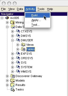
Figure 1: Launching the Build mining activity wizard.
The wizard gives instructions for creating an AI model in five steps:
- Model type selection
- Data selection
- Additional data selection
- Data usage specification
- Model naming
In the Model Type step, select Attribute Importance as the Function Type (Figure 2).
Figure 2: Model type selection step.
In the Data Definition page (Figure 3), do the following:- Select lymph_outcome as the case table.
- Check the "Join additional table with the case table" checkbox. This will launch the select additional data step.
- Select SAMPLE_ID as the key. It is not necessary to have a key column but it helps with performance.
- De-select the columns: FULL_IPI, STATUS, SURTIME. In this example, we only want to use gene expression for predicting outcome.

Figure 3 - Data specification step.
The Additional Data step (Figure 4) allows us to join additional tables to the case table without data replication. As a result we can mine data residing in different tables in a efficient way. For our example, select lymph_bin on the left pane and click on the arrow to move it to the right pane. Then click on the Define hyperlink to define the relationship between lymph_outcome and lymph_bin.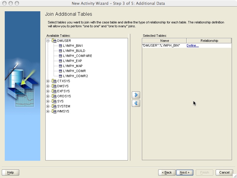
Figure 4 - Additional data specification step.
In the Edit Relationship window (Figure 5) do the following:- Select SAMPLE_ID for the key column mapping
- Select "One to Many" for relationship type. This is a one to many relationship because each SAMPLE_ID has many different gene expression values associated with it.
- Add a one to many mapping specification by pressing the New button

Figure 5: Edit Relationship window.
The New Mapping window (Figure 6) is used to define how information from the additional data source (lymph_bin) should be aggregated before joining it with the case table (lymph_outcome). In this example select GENE_EXP as the value column, GENE_ID as the GROUP BY column, and SUM as the aggregation operation. This specification will return the sum of all the GENE_EXP values for each SAMPLE_ID and GENE_ID combination. The checkbox for sparsity should also be un-checked as lymph_bin is not a sparse data set.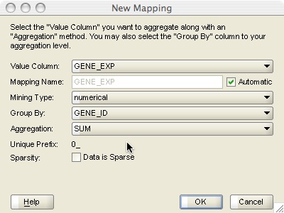
Figure 6: New Mapping window.
In the Data Usage step (Figure 7) the only thing we need to do is to select OUTCOME as the target column. The target column is the one that we want to predict. The other selected columns will be ranked according to how well they can help predict the target column.
Figure 7: Data Usage specification step.
The final step in the wizard is to name the mining build activity. For this example I named it LYMPH_OUTCOME_AI. At this point you can either run mining build activity upon finish or not. Because we have already prepared the data by binning it around the mean, we should uncheck the run upon finish checkbox. After clicking on the Finish button we get the mining activity page (Figure 8). This page lists all the steps that the mining build activity will take to build the AI model. Uncheck the Discretize checkbox, as we have already discretized the data, and then click the Run Activity button.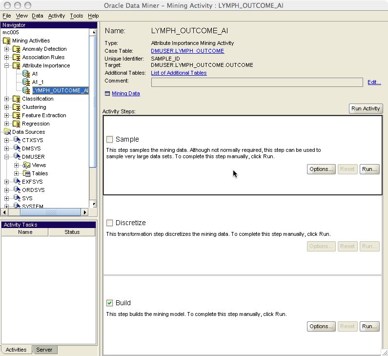
Figure 8: Mining build activity created by wizard.
After the mining activity completes the build task we can review the results by clicking on the Result hyperlink. This brings up the Attribute Importance model viewer (Figure 9). The viewer shows a ranked list of gene IDs (name column) and a bar chart. The list or the bar chart can be used to determine a cut point for filtering genes. One approach would be to select all genes above a big drop in the importance value. For this example, I kept the genes with the top seventeen scores.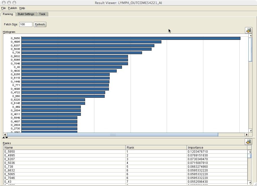
Figure 9: Attribute Importance model viewer.
We can use the information from an AI model in SQL queries using the function get_model_details_AI in the DBMS_DATA_MINING package. For example, the following query returns the top seventeen genes with expression values most correlated with OUTCOME according to the AI model A0:SELECT b.rank, a.gene_id, a.accessionThe inner subquery returns the gene ids ordered by their relevance with respect to outcome. The outer query joins the filtered gene ids with the mapping table to obtain the gene accession information.
FROM lymph_map a,
(SELECT *
FROM (SELECT rank,
attribute_name
FROM TABLE(dbms_data_mining.get_model_details_AI('AI0'))
ORDER BY rank ASC)
WHERE ROWNUM < 18) b
WHERE a.gene_id = b.attribute_name ORDER BY b.rank ASC;
RANK GENE_ID ACCESSION
---------- ---------- ------------------------------
1 5850 M17863_s_at
2 4995 Y09912_rna1_at
3 6207 M18255_cds2_s_at
4 5036 Y12394_at
5 738 D87468_at
6 6632 X99897_s_at
6 7046 J00148_cds2_f_at
6 5065 Z15114_at
7 43 AFFX-HUMGAPDH/M33197_M_at
8 4830 X94910_at
9 6255 M26657_s_at
9 6118 X94628_rna1_s_at
10 1449 L28175_at
11 4098 X07109_at
11 771 D89077_at
12 4722 X85237_at
13 660 D86959_at
17 rows selected.
For models created using Oracle Data Miner we need to modify the query somewhat. For example, for an AI model named AI1 we would write the query as below:
SELECT b.rank, a.gene_id, a.accessionThe reason for this alternative query is that Oracle Data Miner adds a two-character suffix to the name of attributes that come from a nested column. The suffix is added to avoid potential collisions between attribute names derived from multiple nested columns. The name of the AI model associated with a mining build activity can be obtained from the model results Task tab (see Figure 9).
FROM lymph_map a,
(SELECT *
FROM (SELECT rank,
TO_NUMBER(SUBSTR(attribute_name,3)) attribute_name
FROM TABLE(dbms_data_mining.get_model_details_AI('AI1'))
ORDER BY rank ASC)
WHERE ROWNUM < 18) b
WHERE a.gene_id = b.attribute_name ORDER BY b.rank ASC;
After we have selected a subset of genes we can filter the expression data to keep only the values for the selected genes. This can be accomplished with the following query:
CREATE VIEW lymph_small0 ASAlternatively, if the AI model was constructed with Oracle Data Miner we would use the following query:
SELECT c.*
FROM lymph_exp c,
(SELECT a.*
FROM (SELECT *
FROM TABLE(dbms_data_mining.get_model_details_AI('AI0'))
ORDER BY rank ASC) a
WHERE ROWNUM < 14) b
WHERE c.gene_id = b.attribute_name;
CREATE VIEW lymph_small1 AS SELECT c.*
FROM lymph_exp c,
     (SELECT a.*
      FROM (SELECT TO_NUMBER(SUBSTR(attribute_name,3)) attribute_name
            FROM TABLE(dbms_data_mining.get_model_details_AI('AI1'))
            ORDER BY rank ASC) a
      WHERE ROWNUM < 14) b
WHERE c.gene_id = b.attribute_name;


Hi Marcos,
very interesting your blog ... i didn't know, but i think that it will help me a lot.
i'm use data mining in research and now i'm starting to use in commercial softwares. I work in a partner oracle in brazil and here there isn't people work with oracle data mining. We don't find at least.
If i to need of a help, can i find you ?
and a simple question, you know how i can get the matrix of distances that the k-means genereated in ODM ??? i was tring do a tree in other software, but i need of this matrix.
thanks a lot ...
ps* my e-mail is vmuniz@commitconsultores.com.br
Posted by Anonymous |
9/21/2006 04:14:00 PM
Anonymous |
9/21/2006 04:14:00 PM
Hi Vander:
Happy to hear that you like the blog. Let me know if there are topics you would like discussed. No promisses, but I will try to write about it if the topic has broad appeal.
Take a look at my reply at the ODM forum to your question (http://forums.oracle.com/forums/thread.jspa?messageID=1474737??). I have some extra questions.
Regarding help with ODM the ODM forum is a good venue. You will have access to advice from a broad group of people. I, among others in the development team, read and answer questions in the forum frequently.
Regards,
-Marcos
Posted by Marcos |
9/25/2006 09:43:00 AM
Marcos |
9/25/2006 09:43:00 AM
hello sir,
I am vj, I am learning SQL using 2005....can you provide me some websites from where I can download database to get exposure and get realtime exerience on working on a lifescience database using sql....could you please send me the links to my mail ID:
bijoy777@gmail.com.......
Thanks in advance........
regards!!!!!
Posted by DeXtEr |
11/25/2007 02:03:00 AM
DeXtEr |
11/25/2007 02:03:00 AM
Hi VJ,
When you say "SQL using 2005" do you mean MS SQL Server 2005? If this is the case I cannot help you as I am not knowledgeable about that software.
What kind of problems are you interested in working with in life sciences?
Regards,
-Marcos
Posted by Marcos |
12/03/2007 03:35:00 PM
Marcos |
12/03/2007 03:35:00 PM