Time Series Forecasting 2 - Single-step Forecasting
This is Part 2 in a series on time series forecasting - The full series is Part 1, Part 2, and Part 3.
This post, long overdo, covers how to do single-step or open-loop forecasting using the data mining approach described in Part 1 of this series. It describes each step of the methodology with an example and, at the end, compares the results with those from a traditional time series approach.
Single-step forecasting (Part 1) does not use a model's previous predictions as inputs to the model's later predictions. If the previous value of the target is included as input to the model, we can only make forecasts for the next time interval, thus the single-step name. Single-step forecasts can be directly computed using Oracle Data Miner's Apply and Test mining activities or the SQL PREDICTION function.
Methodology
As discussed in Part 1, when modeling time series it is usually necessary to make decisions regarding:
- Variance stabilization and trend removal
- Target normalization
- Lagged attribute selection
After these steps have been taken, it is possible to create a regression model that can be used for forecasting future values of the series.
In order to illustrate the process, let's take a look at an example of non-stationary seasonal time series widely used in the time series literature. The data is provided in the book Time Series Analysis: Forecasting and Control by Box and Jenkins (1976). The series corresponds to monthly international airline passengers (in thousands) from January 1949 to December 1960 (Figure 1).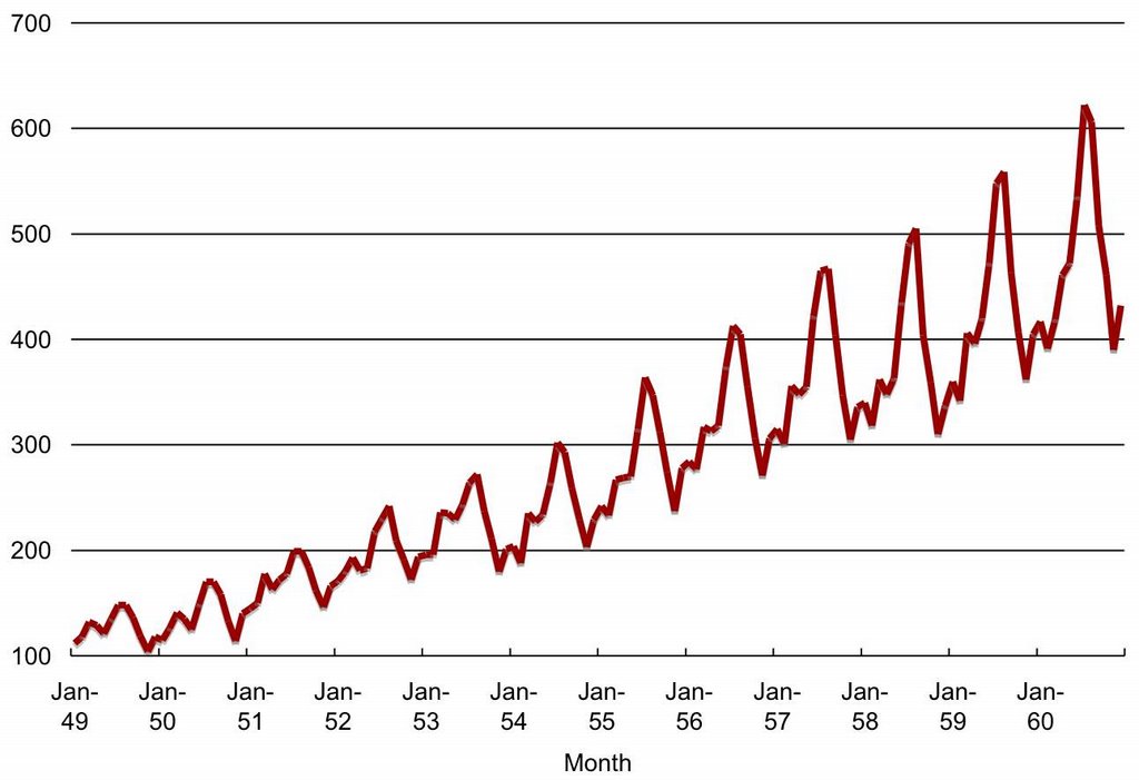
Figure 1: Number of international airline passengers (thousands) per month.
Preparing the Series
Before modeling a time series we need to stabilize the series. That is, remove trends from the mean and from the variance. If the mean has a trend then the average value of the series either steadily increases or decreases over time. If the variance has a trend then the variability of the series steadily increases or decreases over time. Ideally, what we are looking for is the series to be bouncing up and down a fixed value (the mean) and with about the same amount of bouncing over time. The series in Figure 1 has both a trend in the mean, it steadily increases over time, and the variance, the size of the swings in the series also steadily increases over time.
First we stabilize the variance. This can be done by applying a Box-Cox power transform. This transform has the following form: y(h) = (y^h - 1) / h, if h is not equal to 0 and y(h) = log(y) if h is 0. In general, the LOG transform (h=0) is a good choice for removing increasing variability. Figure 2 shows the transformed series after the LOG transform. The upward trend over time is still visible but the amount of variation in the series is about the same throughout the series.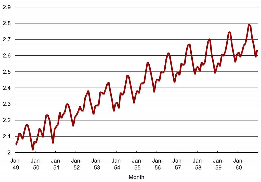
Figure 2: Log transformed series.
After stabilizing the variance, we can remove the remaining trend by differencing the series by subtracting the value of the series at time t from the value in the previous time period t-1 (Part 1). This process can be repeated until the trend disappears. Alternatively, we can add a time index (e.g., elapsed time from a fixed date) as one of the predictors. Figure 3 shows that the upward trend has been removed from the data after differencing the LOG transformed series once.
Figure 3: First order differencing after log transformation.
We can easily stabilize the series (variance and mean) using SQL. I used, for the above transformations, the SQL LOG function (variance stabilization) and the LAG analytical function (differencing) as follow:CREATE VIEW airline_xfrm ASThe inner query stabilizes the variance using the LOG transformation. The outer query implements first order differencing. I am keeping the untransformed series (passengers) around to compute model quality later on. If we needed higher order differencing we would repeat the outer query. For example, the following query does a second order differencing:
SELECT a.*
FROM (SELECT month, passengers,
tp - LAG(tp,1) OVER (ORDER BY month) tp
FROM (SELECT month, passengers, LOG(10,PASSENGERS) tp
FROM airline)) a;
CREATE VIEW airline_xfrm1 AS
SELECT a.*
FROM (SELECT month, passengers,
             tp - LAG(tp,1) OVER (ORDER BY month) tp
      FROM (SELECT month, passengers,
                   tp - LAG(tp,1) OVER (ORDER BY month) tp
            FROM   (SELECT month, passengers, LOG(10,PASSENGERS) tp
                    FROM   airline))) a;
This can also be done in Oracle Data Miner (ODMR) using the Compute Field transformation under the Data-Transformation menu. In this case, first create a view with a new column with the LOG transformed value. Next, create a new view using the LAG transformation.
After stabilizing the series we can optionally normalize it. It is usually useful to normalize the target for SVM regression. This helps speed up the algorithm convergence. For time series problems, the target should be normalized prior to the creation of the lagged variables. If done afterwards, we should use the range of values in the original series for setting the normalization parameters. Normalization can be done using ODMR, DBMS_DATA_MINING PL/SQL package, or the data mining Java API. In the case of ODMR the normalization transformation is under the Data-Transformation menu. For this example, I selected z-score normalization. This transformation subtracts the mean of the series from each sample and then divides the result from the standard deviation. For the airline_xfrm view we have AVG(tp)= 0.003919158 and STDDEV(tp)= 0.046271162. The view with the normalized data is as follow:
CREATE VIEW airline_norm AS
SELECT month, passengers, (tp - 0.003919158)/0.046271162 tp
FROM   airline_xfrm;
Selecting Lagged Variables
Before building a model we need to select which lag values of the prepared series to use as predictors of future values. In the case of the data mining approach described in Part 1, this is equivalent to selecting a time window and including all the lag values in that window. Prior knowledge about the activity represented by the series can provide an initial clue. For example, for a monthly series, we could select a window of size 12 if we know that the series has a similar behavior on yearly basis. It is also useful to analyze the autocorrelations in the series and chose a window size that includes the largest autocorrelation terms.
Figure 4 shows the first twenty autocorrelations coefficients for the airline series. The largest autocorrelation term is at lag 12. This matches the expected behavior that airline travels have a strong yearly seasonal effect. Based on this analysis, we may want to include as predictors all the lags in a window of size 12.
Figure 4: First twenty autocorrelation coefficients for the airline data.
Autocorrelations can be easily computed using the SQL CORR and LAG analytical functions. The autocorrelation of the airline series with its first lag can be computed as follow:SELECT CORR(ts,tp)The xcorr function below can be used to compute all autocorrelations, over a window of p_max_lag size, for a series in the p_base_col column and sequence index (e.g., the time column) given in the p_seq_col column. In fact, the function returns the cross-correlation between any two columns (p_base_col and p_lag_col). The autocorrelation is computed as a special case when p_base_col and p_lag_col are the same.
FROM (SELECT tp, LAG(tp,1) OVER (ORDER BY month) ts
FROM airline_norm);
CREATE OR REPLACE PROCEDURE xcorr(p_in_table VARCHAR2,Modeling
p_out_table VARCHAR2,
p_seq_col VARCHAR2,
p_base_col VARCHAR2,
p_lag_col VARCHAR2,
p_max_lag NUMBER) AS
v_stmt VARCHAR2(4000);
v_corr NUMBER;
BEGIN
v_stmt:= 'CREATE TABLE ' || p_out_table ||
'(lag_num NUMBER, correlation NUMBER)';
EXECUTE IMMEDIATE v_stmt;
FOR i IN 1..p_max_lag LOOP
v_stmt:=
'SELECT CORR(' || p_base_col || ', lag_val) ' ||
'FROM (SELECT ' || p_base_col || ',' ||
'LAG(' || p_lag_col || ',' || i || ') ' ||
'OVER(ORDER BY ' || p_seq_col || ') lag_val ' ||
'FROM ' || p_in_table || ')';
EXECUTE IMMEDIATE v_stmt INTO v_corr;
v_stmt:='INSERT INTO ' || p_out_table ||
' (lag_num, correlation) VALUES(:v1, :v2)';
EXECUTE IMMEDIATE v_stmt using i, v_corr;
END LOOP;
END;
/
SHOW ERRORS;
After preparing the series and selecting the lagged variables we are ready to build a model to forecast future values of the series. The starting point is the prepared series computed in the above airline_norm view. The month column is a sequence ranging from 1 to 144 going up with time. The first row is NULL as we differenced the original series once.
First we need to create a view with the twelve lagged variables:
CREATE VIEW airline_lag ASWe can also create this view using ODMR's Compute Field wizard.
SELECT a.*
FROM (SELECT month, passengers, tp,
LAG(tp, 1) OVER (ORDER BY month) L1,
LAG(tp, 2) OVER (ORDER BY month) L2,
LAG(tp, 3) OVER (ORDER BY month) L3,
LAG(tp, 4) OVER (ORDER BY month) L4,
LAG(tp, 5) OVER (ORDER BY month) L5,
LAG(tp, 6) OVER (ORDER BY month) L6,
LAG(tp, 7) OVER (ORDER BY month) L7,
LAG(tp, 8) OVER (ORDER BY month) L8,
LAG(tp, 9) OVER (ORDER BY month) L9,
LAG(tp, 10) OVER (ORDER BY month) L10,
LAG(tp, 11) OVER (ORDER BY month) L11,
LAG(tp, 12) OVER (ORDER BY month) L12
FROM airline_norm) a;
Next we create the training dataset as a subset of the rows in airline_lag. Because we want to test the model's forecasting capability we should train on older data samples and held aside, for testing, the most recent samples in the series. Samples 132-144 are used for the test data set. We also need to filter the first 13 rows as some of the lagged variables have NULLs for these rows. The following view creates the training data set:
CREATE VIEW airline_train ASFinally we build the model using either ODMR or one of the data mining APIs. For this example, I used the PL/SQL API and the default settings for the SVM regression algorithm:
SELECT month, tp, L1, L2, L3, L4, L5, L6, L7, L8, L9, L10, L11, L12
FROM airline_lag a
WHERE month > 13 AND month < 132;
BEGINThis statement creates an SVM regression model named airline_SVM using the view airline_train as the training data.
DBMS_DATA_MINING.CREATE_MODEL(
model_name => 'airline_SVM',
mining_function => dbms_data_mining.regression,
data_table_name => 'airline_train',
case_id_column_name => 'month',
target_column_name => 'tp');
END;
Figure 5 displays the residual plot for the training data. The residuals are computed as the difference between the prediction and the actual value for the series. Ideally we want the residuals (Y-axis values) to be randomly distributed around zero with no discernible trends. The plot shows that the model does a good job capturing the process underlying the time series.

Figure 5: Residual plot.
Forecasting
To create forecasts we only need to apply the model to new data. For example, applying the model to the airline_lag view generates one-step ahead forecasts for both the training data (samples 1-131) as well as the held aside test data (samples 132-144). The following query accomplishes that:
SELECT month, passengers,However, because the model predictions reflects the transformed data, we cannot compare the predictions with the original values. In order to do so we need to reverse the transformations to bring the results back to the original scale of the data. The steps below list the transformations that need to be reversed as well as how to reverse them. These steps should be done in order:
PREDICTION(airline_svm USING a.*) pred
FROM airline_lag a;
- Normalization: multiply by the standard deviation (0.046276747) and add the mean (0.00409976)
- Differencing: add the previous value of the series to the result from the previous step
- Log: raise 10 to the result of the previous step
CREATE TABLE airline_pred ASThe innermost query undoes the normalization and computes the log of the original series. The latter is needed for undoing the differencing operation. The subquery with the LAG function undoes the differencing step used to remove the trend in the mean of the original series. The outermost query undoes the LOG transformation used for stabilizing the variance.
SELECT month, passengers, power(10, pred) pred
FROM (SELECT month, passengers,
pred + LAG(lp,1) OVER (ORDER BY month) pred
FROM (SELECT month, passengers, LOG(10, passengers) lp,
(PREDICTION(airline_SVM USING a.*)
* 0.046271162 + 0.003919158) pred
FROM airline_lag a));
Figure 6 shows the original data, the model predictions, and the residuals for the whole time period (month 1-144). Due to the use of first order differencing, we do not have a prediction for the first time period (month 1).
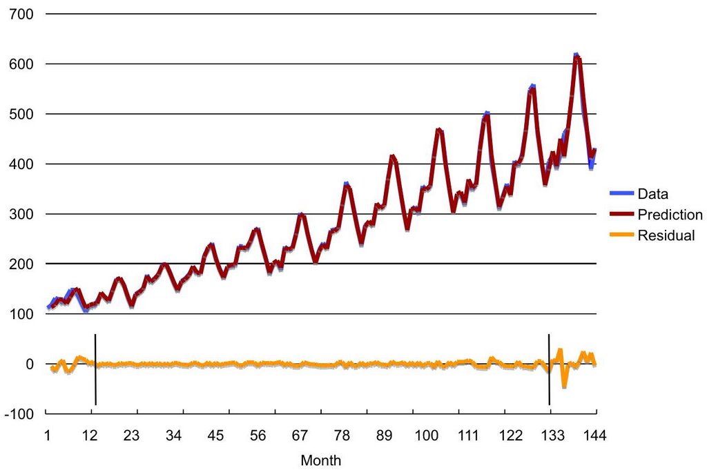
Figure 6: Data, predictions, and residuals.
The two vertical bars in the residual series mark the beginning and the end of the samples used for training the model. Samples to the left of the first bar contain NULL values for some of the lagged variables used as inputs to the model. The predictions for this period are a bit off as some of the inputs are missing. Samples to the right of the second bar are the held aside samples used for measuring the model's generalization capabilities. Note that the model output for these samples are one-step ahead forecasts of data unseen during training of the model.
Comparison with Other Techniques
How well does the data mining approach described above compare with other techniques? Table 1 presents the Root Mean Squared Error (RMSE) and Mean Absolute Error (MAE) for the training and the forecast (test) data sets for the data mining approach (SVM) and a linear autoregressive model (AR).
| Model | RMSE Training | MAE Training | RMSE Test | MAE Test |
| SVM | 3.7 | 3.2 | 18.9 | 13.4 |
| AR | 10.1 | 7.7 | 19.3 | 15.9 |
The data mining approach performed well. It had smaller RMSE and MAE in the training and the forecasting (test) data sets.
The next post in this series will show how to do multi-step forecasting. The full series is Part 1, Part 2, and Part 3.
10/26/06 - Edits
In the airline example described above, the normalization shift and scale parameters were computed using the whole data. A better methodology would be to use only the training data for computing these parameters. This alternative normalization scheme also impacts the results for the airline example described in Part 3 as the latter builds on the transformations described in Part 2.
I have changed the normalization in the above queries so that the parameters are computed using only the training data time period. The results for the RMSE and MAE did not change with the new normalization scheme.
Readings: Business intelligence, Data mining, Oracle analytics
Labels: Time Series


What are using the create the charts you have displayed here?
Posted by Anonymous |
3/30/2006 10:08:00 PM
Anonymous |
3/30/2006 10:08:00 PM
I used MS Excel. I've cut and pasted the data from Oracle Data Miner directly into Excel.
Posted by Marcos |
3/30/2006 11:11:00 PM
Marcos |
3/30/2006 11:11:00 PM
I have been asked if I could give a link to the airline data. Here are a couple of links to the data:
Excel spreadsheet.
Text file. It is the last data set in the file (the Grubb-Mason airline passenger time series). This is not in a convenient format but the link is less likely to disappear.
Posted by Marcos |
5/24/2006 06:45:00 AM
Marcos |
5/24/2006 06:45:00 AM
Mr Campos,
I hope you don't mind, but I will need to use some of your text as a reference in a statistics paper "prior knowledge about the activity represented by the series can provide an initial clue. It is also useful to analyze the autocorrelations in the series and chose a window size that includes the largest autocorrelation terms".
In a regression analysis, what is the best value of Lagged data and how can the differences in R values be explained?
Posted by Anonymous |
5/27/2006 02:16:00 PM
Anonymous |
5/27/2006 02:16:00 PM
The best value for the maximum lag for each attribute needs to be determined for each data set. There have been many criteria proposed in the literature for determining the autoregressive lag length of time series variables. Here are some references on the topic: "Non-parametric Lag Selection for Time Series", "Lag Selection in Time Series Data", and "Which Lag Length Selection Criteria Should We Employ?."
It is important to notice that the approach I described used the SVM regression algorithm for learning the autoregressive model. The above references are mostly discussing linear autoregressive models. The SVM approach differs in two ways: the model can be non-linear (gaussian kernel case) and, more importantly, it is not estimated the same way as the traditional linear autoregressive model. The traditional model is estimated by minimizing the sum of squared errors (least squares, maximum likelihood) while the SVM model algorithm minimizes structural risk (with a epsilon-insensitive loss function in my examples). Lag selection criteria (e.g., AIC), in general, assume a traditional linear autoregressive model. As such, they might not be applicable to the SVM approach.
Lag selection for SVM approach to time series forecast is similar to that in neural networks. Usually, this is done by inspection of autocorrelation and partial autocorrelations. This is the method I described in the paper. A nice feature of SVM, because it tries not to overfit the data, is that the error should go down as we increase the size of the window until we reach the optimum window size (optimum maximum lag). Afterwards, it should remain constant. As a rule of thumb we can try a couple of models with increasing window sizes and select the one that achieves the smallest error before the error remains constant. Murkherjee et al found that this approach worked well for low dimensionality kernels. For high dimensional kernels, they found that, because of a slight overfit to the data, this approach would select a larger window size than necessary, but not by much.
Finally, regarding R (correlation coefficient), it has an assumption that the model is a linear model. SVM regression in not a linear model if the kernel, as in the examples in the post, is not the linear kernel. For non-linear models R is not applicable directly (see here and here).
Posted by Marcos |
5/29/2006 06:30:00 AM
Marcos |
5/29/2006 06:30:00 AM
Hi Marcos,
I have noticed that you are using the testing data itself while making the prediction for test data. "CREATE TABLE airline_pred .."
Doesn't that cause a bias?
Posted by memilthegreat |
5/28/2007 07:19:00 PM
memilthegreat |
5/28/2007 07:19:00 PM
Hi Husnu:
Thanks for the comment. This is an important point. In this case it is not a problem because I am doing one-step ahead forecast. During the testing phase the model has available to it previous values of the series but the next one (the one to forecast). So to forecast at time t+1 I can use values of the series all the way to time step t. In the case of multi-step forecasting (part 3 post) then I cannot use any of the values in the test data.
Posted by Marcos |
5/29/2007 10:18:00 AM
Marcos |
5/29/2007 10:18:00 AM
Thanks for your answer. Then can we say that in practice multi-step forecasting is more useful. Since usually we don't know the data that will be predicted. Right?
Posted by memilthegreat |
5/29/2007 05:23:00 PM
memilthegreat |
5/29/2007 05:23:00 PM
Actually both types of forecast are very useful. It is really a matter of how far ahead in the future you need to forecast. Ideally, it would be better to do one-step ahead forecast if you can as you don't need to use the model's previous forecasts (guesses) as input for future ones.
In both scenarios you do not have the data for the period that you want to forecast. In my example I had the data for many periods ahead. But in a real situation the analyst would only have data about the past. He would forecast the next time period and would evaluate the forecast once he received the new data.
This is not uncommon. For example, a publishing company may need to forecast what will be the demand for its magazines for the coming week. It will then print enough magazines to cover the estimated demand. It will do it every week one step at a time. It will only know how good the forecast was after the end of the week.
Posted by Marcos |
5/29/2007 08:10:00 PM
Marcos |
5/29/2007 08:10:00 PM